I like data. Yes, I know, I’m a nerd.
It has been a little over a year since I deployed some indoor and outdoor temperature sensors in and around my home. They have been taking a reading every 10 minutes for that entire year (except for a few brief gaps for various reasons), logging well over 250,000 readings at last count.
For this post, I am exploring different ways to look at a year’s worth of these temperature readings. Again, I’m doing this just because I have an interest in collecting, analyzing, and visualizing data. Though the data may not be as interesting to other folks, I hope this post is of at least passing interest to folks who also just like data. The post demonstrates the power of data slicing.
All plots in this post use temperature readings taken between Nov 1 2025 and Oct 31 2026. I have slightly more data than that, but I decided to limit the data used to just cover a full year, mostly because the data before Nov 1 2025 had a couple more brief outages. The temperature data for this post was collected from sensors in the following locations:
| Location | Description | Data Points |
|---|---|---|
| Outside | The air temperature from a sensor deployed in my backyard, away from my house, in the shade | 52,547 |
| Pool | The water temperature from a floating thermometer in my backyard pool. It is tied to the side of my pool, situated to always be in the shade | 51,518 |
| Attic | The air temperature from a sensor deployed in the attic of my 2-story home | 52,547 |
| Studio | The air temperature from a sensor in my home studio, which is located in a second-story room in my home. | 52,547 |
For some reason, the WiFi connection to the Pool sensor is less reliable than for the other sensors, so it has a few more gaps in the data.
The first few months of this same data were used in the Backyard Data Science series of posts. The same data science tools were used.
All the Data
Here are all the recorded temperatures for Outside, Pool, Attic, and Studio. No averaging or smoothing.
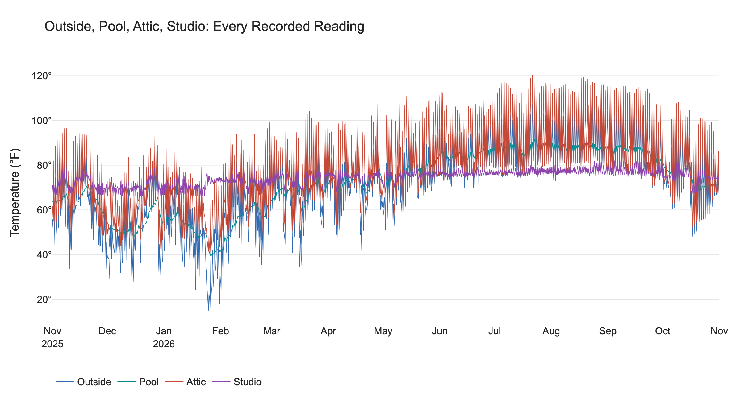
Each line follows the original readings within the selected period. Missing intervals are left as gaps
At this scale, the daily rise and fall of daytime warming and nighttime cooling makes the data a bit hard to see and interpret.
The Studio is the quiet purple line through the middle. Across its entire record, it stayed between 65.3 and 82.0 degrees F, because that is the range that I had set on my upstairs thermostat. Meanwhile, my Attic (whose floor is separated from the ceiling of my upstairs Studio by about a foot of wood, drywall, and insulation) reached 120.4 degrees F, while its lowest recorded temperature was 39.7 degrees. The Pool water temperature was likewise quieter than the Outside temperatures just because a body of water has a ’thermal inertia’ that resists sudden swings in temperature. The Pool ranged only between 39.4 and 91.8 degrees F, while the Outside air temperature (taken about 6 feet from the pool) ranged from 14.9 to 110.7 degrees.
Here is a summary chart of the recorded temperature extremes:
| Location | Lowest reading (F) | Highest reading (F) | Average daily high-minus-low (F) |
|---|---|---|---|
| Studio | 65.3 | 82.0 | 4.4 |
| Attic | 39.7 | 120.4 | 28.6 |
| Outside | 14.9 | 110.7 | 21.5 |
| Pool | 39.4 | 91.8 | 2.4 |
Daily Highs and Lows
To make the seasonal pattern easier to see, I reduced each calendar day to two numbers: its highest recorded temperature and its lowest recorded temperature, and I gave each of the four locations its own panel. A thin vertical stroke runs from each day’s low to its high. The length of the vertical line shows how much the temperature varied that day.
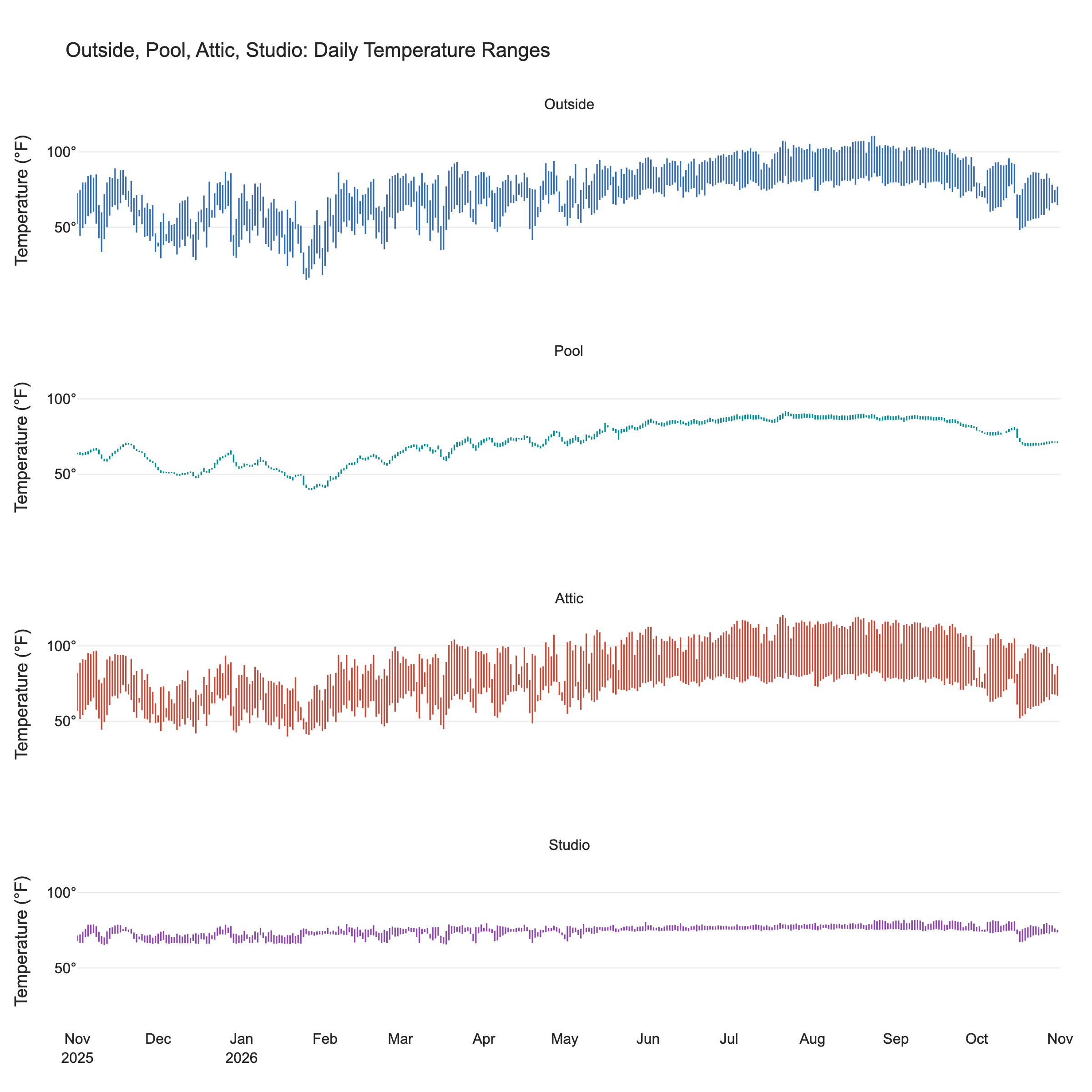
All four panels use the same dates and temperature scale, so their stroke lengths can be compared directly.
The main take-away from these plots is that the Outside, Attic, and Pool temperatures all follow roughly the same seasonal variation, though at different amplitudes. However, my Studio is inside my house, which has an HVAC system to keep the temperature within a narrow band even when the outside temperatures are doing something dramatic (at least when the electricity stays on, which it thankfully did this year). The variations on the Studio plot have more to do with how I’ve set my thermostat than what the outside weather is doing.
Here is the pool on its own temperature scale, rather than the wider scale needed to include all four sensors.
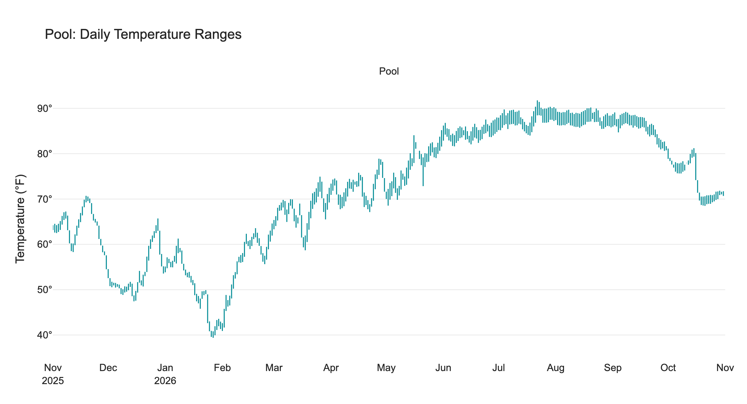
The same low-to-high strokes show the pool’s comparatively small daily temperature swings on an expanded scale.
The Pool’s average daily high-to-low water temperature range was about 2.4 degrees F, compared with 21.5 degrees for the Outside air temperature. Water stores a great deal of heat, so a pool does not usually follow every quick change in air temperature. A body of water provides a natural high-frequency filter on the temperature data.
The Pool temperature is affected by more than just the Outside air temperature; sunlight, evaporation, wind, rain, circulation, and running the pool heater can affect the water temperature. These plots show what the sensor recorded; separating the causes takes more than a temperature graph. See the Backyard Data Science series of posts for far more details.
Smoothed Daily Temperatures
For this plot, I first averaged the actual 10-minute readings within each calendar day, then applied a centered seven-day rolling average to those daily means. Neighboring points share six days of data, so this is a smoother view - it still averages out brief hot or cold spells.
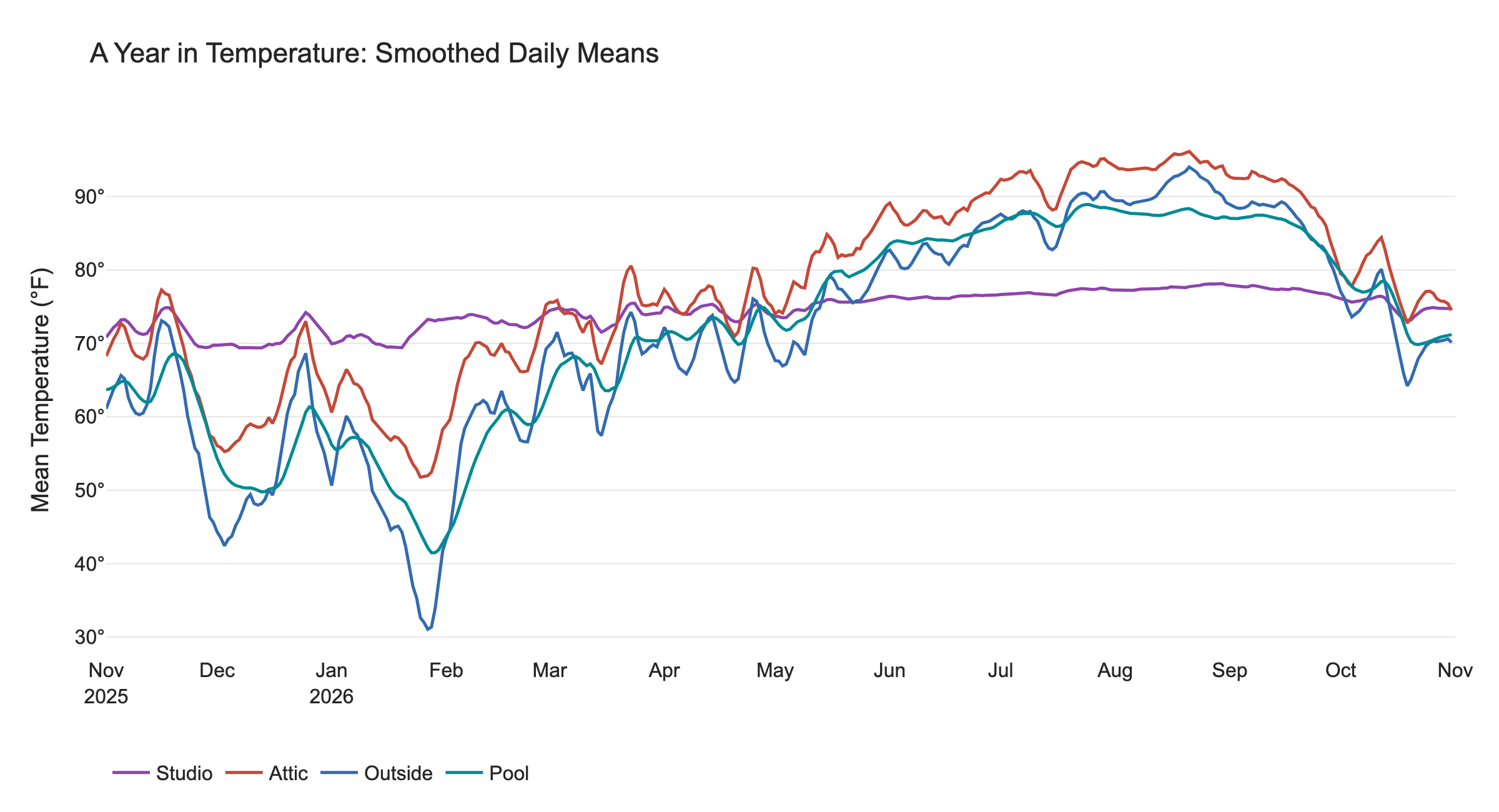
All four smoothed daily averages on a single temperature scale. The smoothing window covers 7 days, and moves forward one day at a time.
From this graph, you can note that during the winter months (e.g., Dec–Feb) the Outside temperature is generally coldest, the Pool is a bit warmer, then the Attic is warmer still, then the Studio (which stays nearly the same all year). But during the summer months (Jun-Aug), the Attic is warmest, the Outside air is a bit cooler, then the Pool, then the Studio. Here’s a Mermaid flowchart showing the temperature rankings in winter and summer:
flowchart TD
    subgraph WINTER["❄️ WINTER (Dec–Feb)"]
        direction TB
        W1["Coldest: Outside"]
        W2["Pool"]
        W3["Attic"]
        W4["Warmest: Studio"]
        W1 --> W2 --> W3 --> W4
    end

    subgraph SUMMER["☀️ SUMMER (Jun-Aug)"]
        direction TB
        S1["Warmest: Attic"]
        S2["Outside"]
        S3["Pool"]
        S4["Coolest: Studio"]
        S1 --> S2 --> S3 --> S4
    end

    style W1 fill:#9CCBFA,stroke:#3978B8,color:#123
    style W2 fill:#B8D9F5,stroke:#3978B8,color:#123
    style W3 fill:#F5CBA7,stroke:#C47A36,color:#123
    style W4 fill:#F9D5A7,stroke:#C47A36,color:#123

    style S1 fill:#F4A261,stroke:#C45D16,color:#123
    style S2 fill:#F6BD80,stroke:#C47A36,color:#123
    style S3 fill:#B8D9F5,stroke:#3978B8,color:#123
    style S4 fill:#D5E8F6,stroke:#3978B8,color:#123
Note: The Studio is nearly constant throughout the year, so its relative ranking changes depending on the season.
A Year, Folded
The charts above reduce many measurements to daily ranges or means. A heatmap keeps all the individual readings but lays them out by date and by time of day, making both the seasonal sweep and the daily rhythm easier to see. The data is folded day-by-day so that readings taken at the same time of day stack vertically on top of each other.
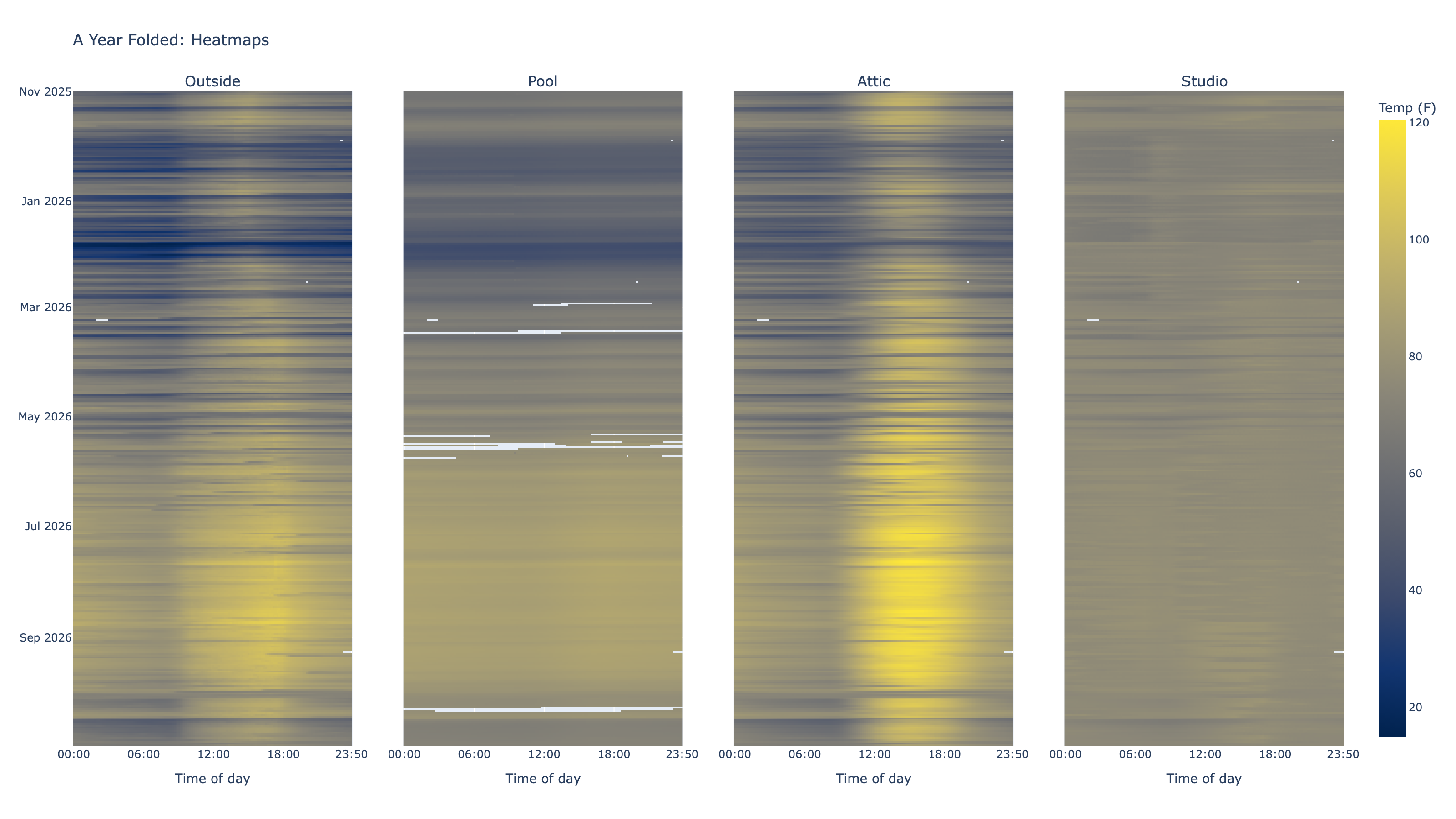
Each colored cell represents one recorded ten-minute reading on a shared color scale; blank cells are missing readings.
The broad seasonal bands are clear, as are the repeated day-and-night cycles. The Attic’s summer colors reach hotter values than the other locations, while the pool changes more gradually. The Studio plot is very bland, the cells are almost all the same color compared to the other plots.
Here the Studio gets its own color range, so that the slight variations in the Studio temperatures stand out:
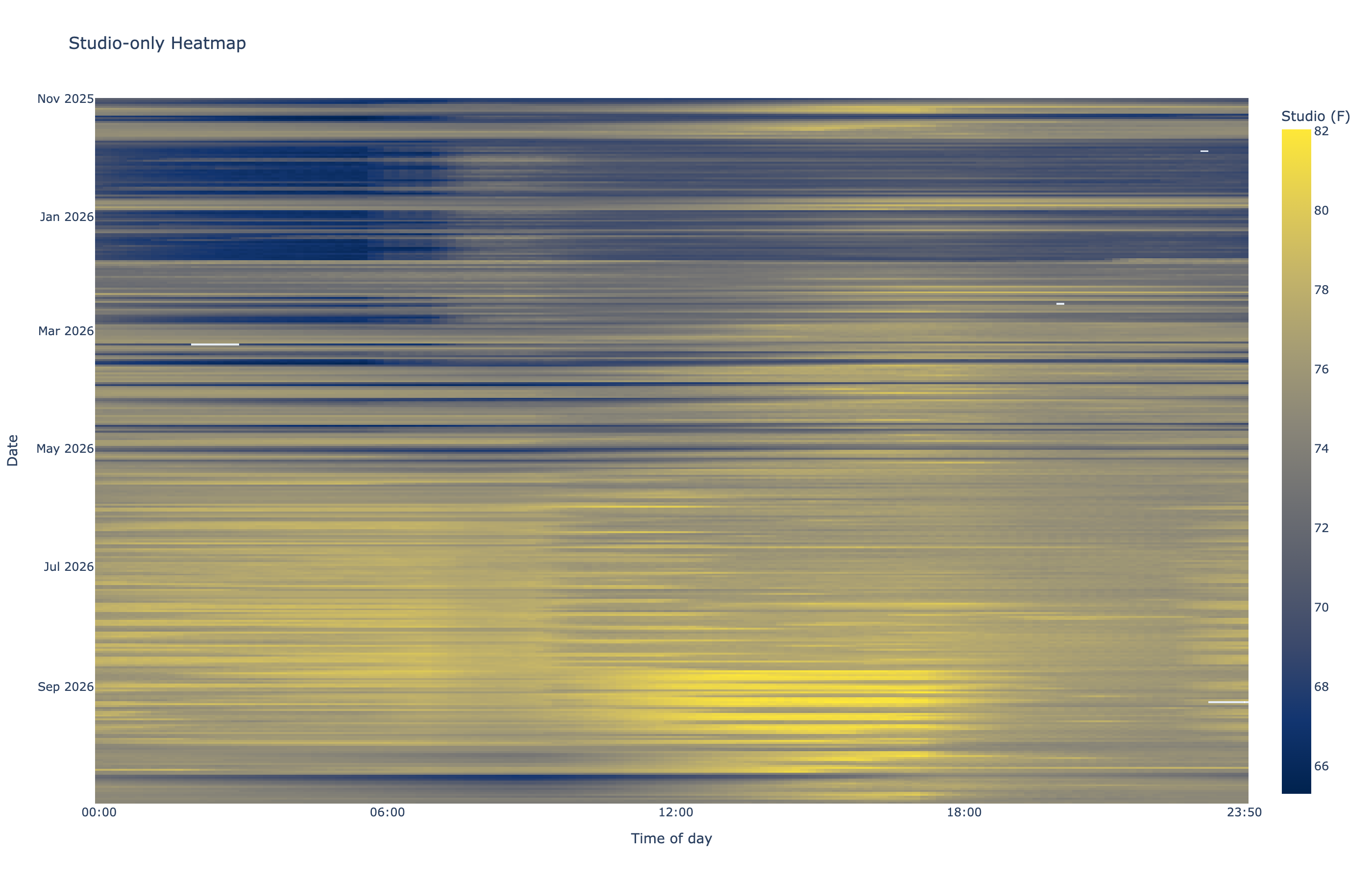
The scale runs from 65.3 to 82.0 degrees F, so the Studio’s smaller variations are visible.
From this plot, I can actually pick out dates when I adjusted my smart thermostat to affect the Studio temperatures. I won’t bore you with details, but the thermostat is configured to allow setting a different temperature for 4 intervals each day, with sleep, wake, daytime, and evening time periods. I can pick out the vertical bands of each time interval on the plot.
A Typical Daily Cycle, by Season
Instead of plotting every day’s traces, I grouped hourly means by season and clock hour. The shaded band spans the middle half of the observed hourly values.
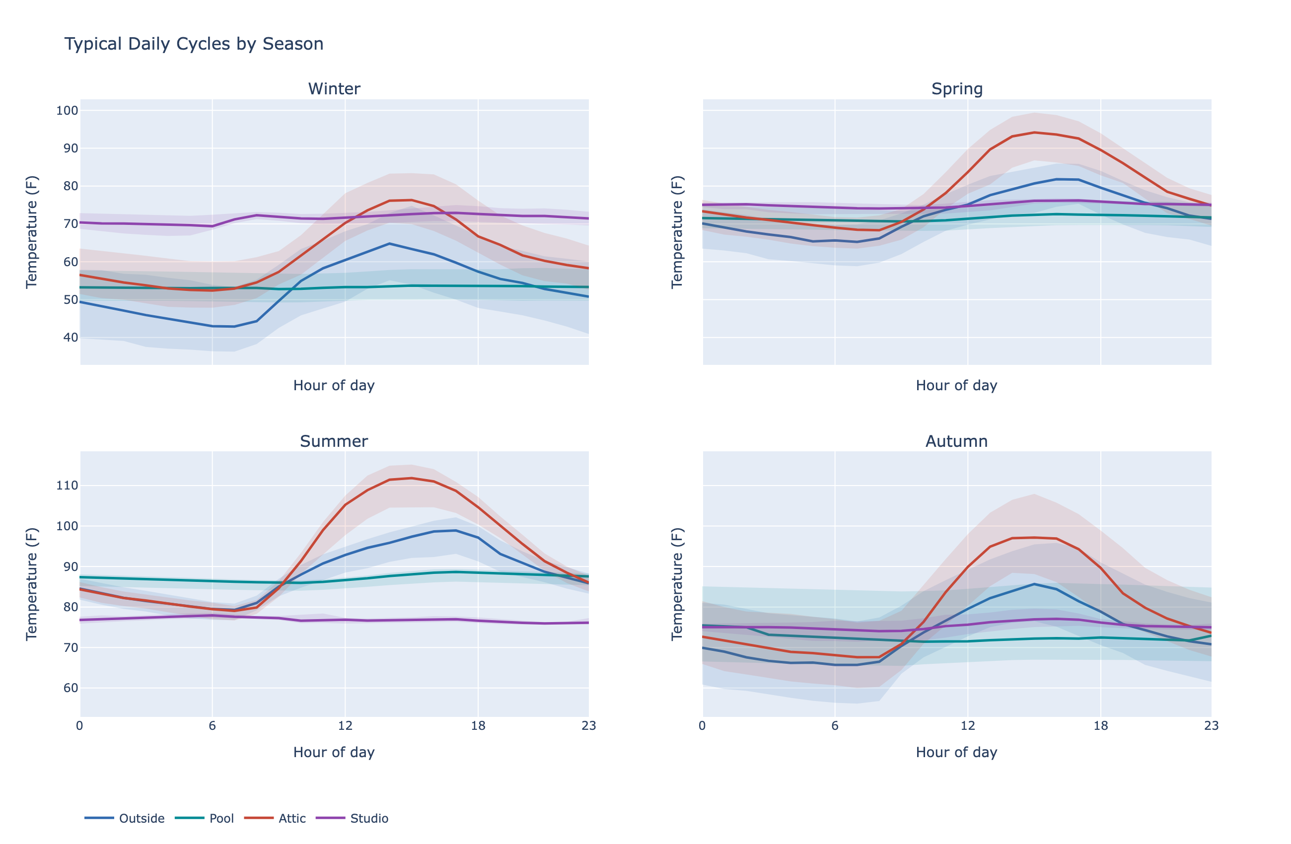
Each panel is a season. A wider band means more variation between observed temperatures at that time of day.
Note from this plot that during the afternoon hours, the Attic is usually warmest, no matter the season.
Attic Vs Studio
The next two heatmaps subtract simultaneous readings. Positive values mean the first-named sensor was warmer; negative values mean it was cooler.
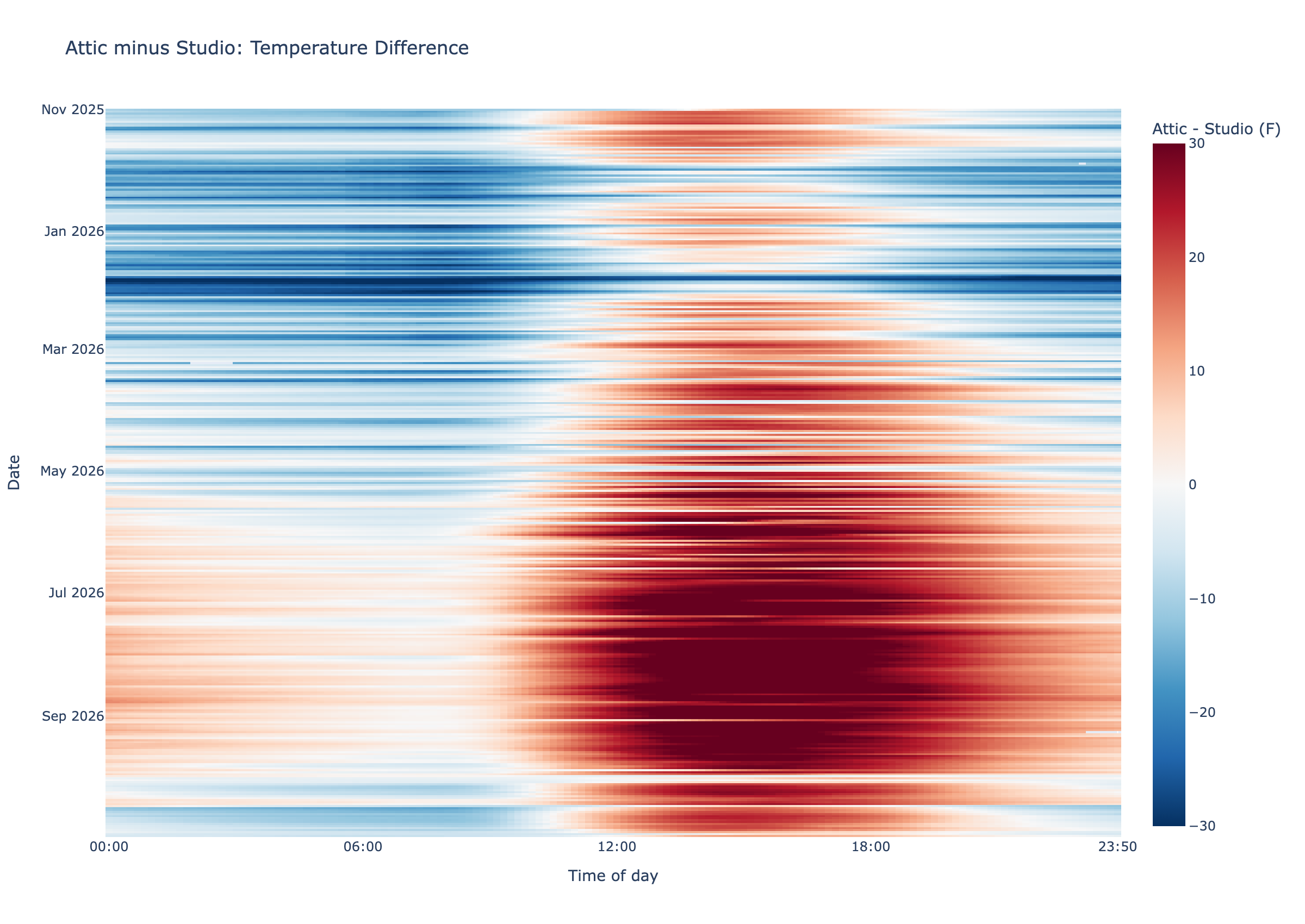
Red means the Attic reading was warmer than the Studio at the same timestamp; blue means it was cooler.
The fact that the Attic was warmer than my Studio in the afternoon stands out on this plot, especially during the summer months.
Pool Vs Outside
The same matched-reading approach shows how the pool relates to the outdoor sensor throughout the year.
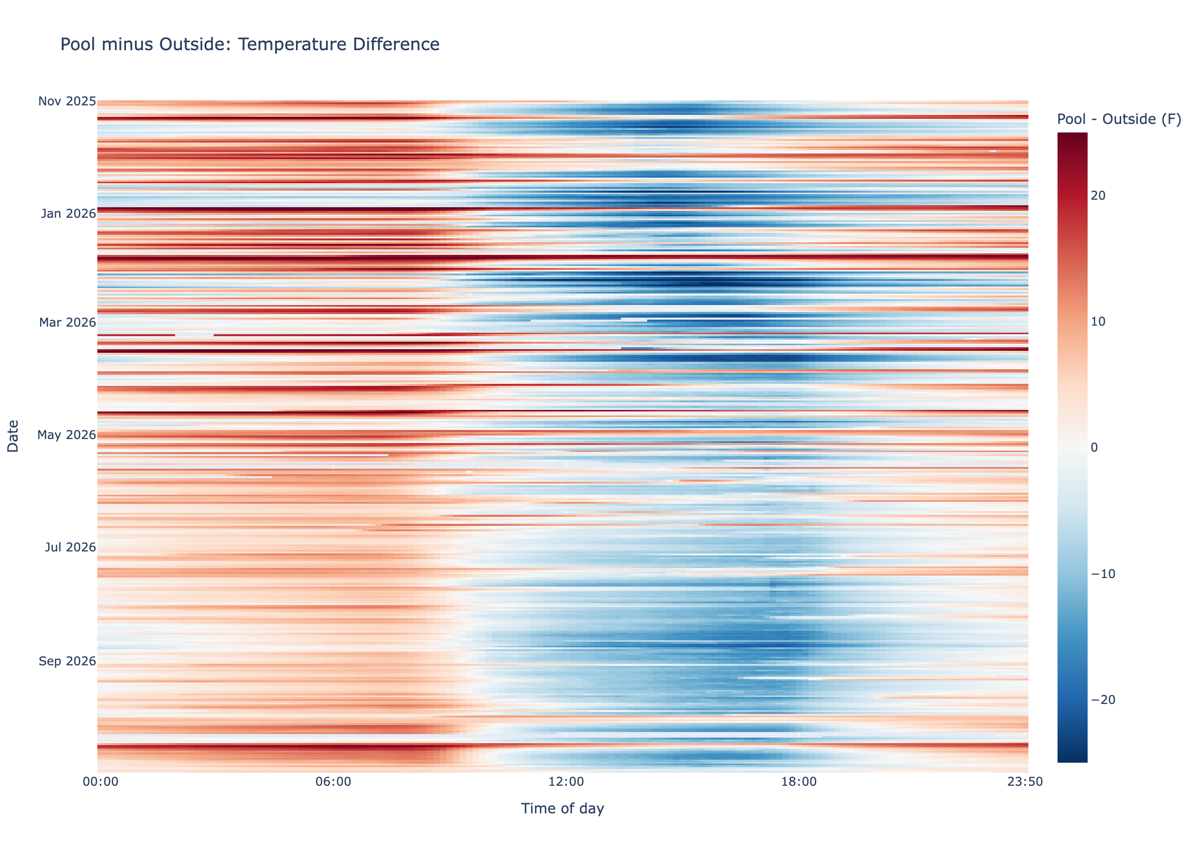
Red means the pool reading was warmer than Outside at that instant; blue means it was cooler.
The Pool tends to be slightly warmer than Outside at night and slightly cooler during the day, no matter the season.
Pool Vs Air Across the Seasons
Each dot below compares one day’s Pool mean temperature with the Outside mean temperature, both calculated from the same timestamps. The dotted diagonal marks equal temperatures.
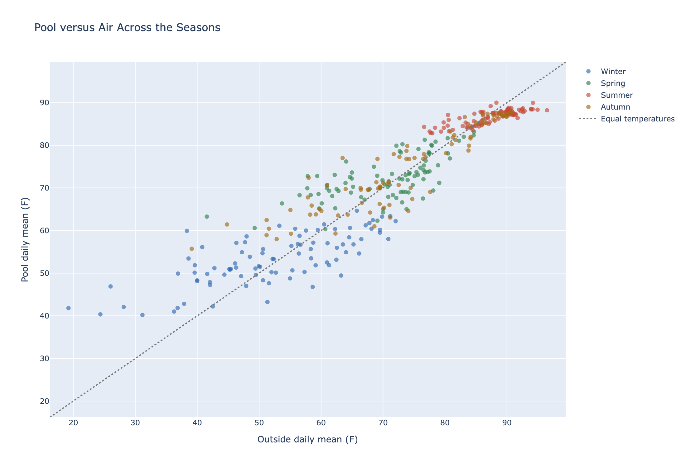
Points below the diagonal mean the Pool was cooler than Outside; points above it mean the Pool was warmer. Season colors show the annual pattern.
On average, the Pool was about 1.0 to 1.8 degrees F warmer than Outside in winter, spring, and autumn, and about 0.8 degrees F cooler in summer. The seasonal change is modest next to the much larger daily swings in the air temperature.
One Fast Change, Up Close
This close-up marks the largest observed 24-hour drop in hourly average Outside temperature.
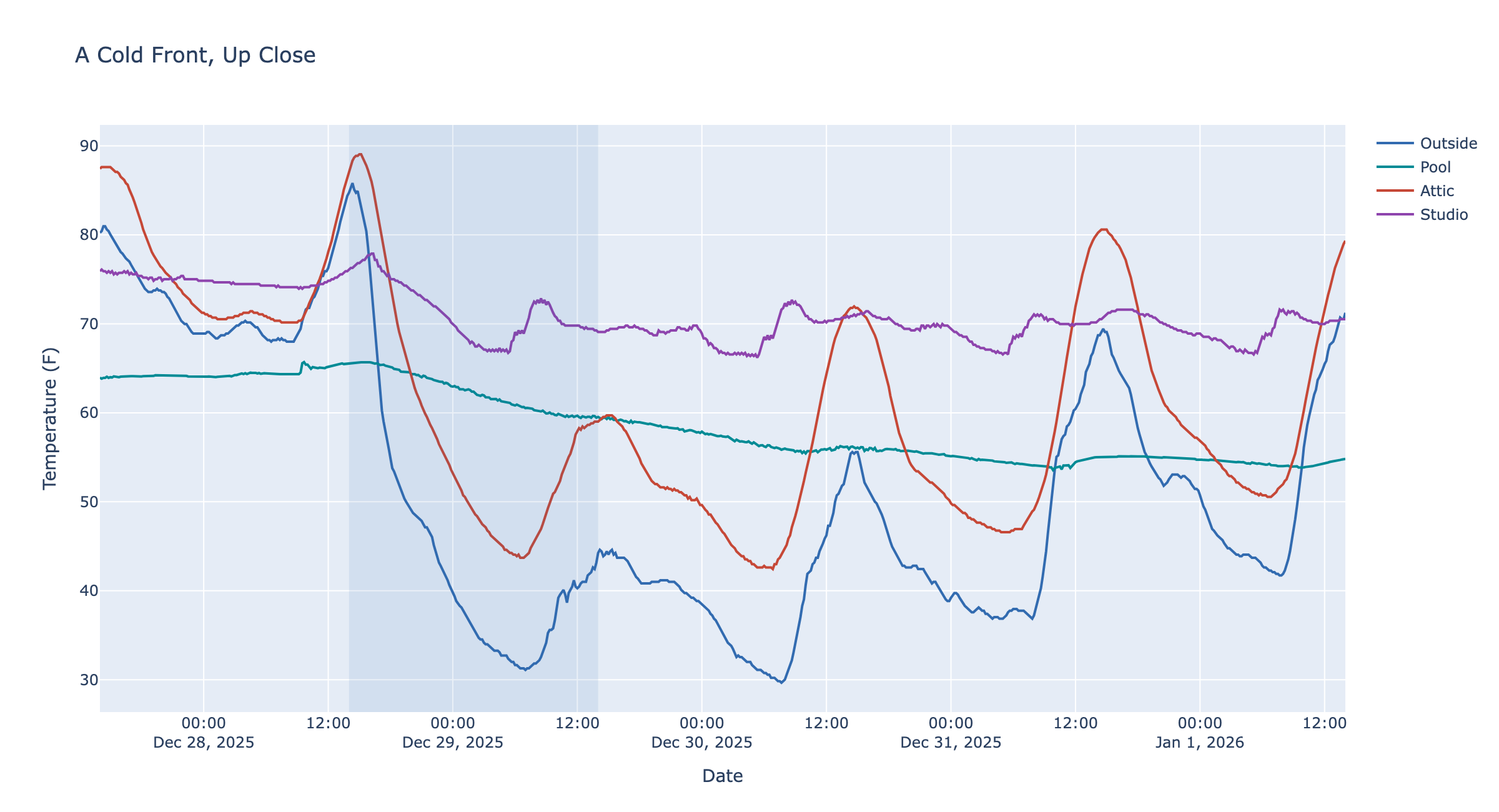
From December 28 to December 29, 2025, the Outside hourly mean fell 40.8 degrees F in 24 hours, from 85.1 to 44.3 degrees F. The shaded interval marks the endpoints used for that comparison.
The other traces make the different responses visible over the same event. The Pool moves less abruptly than the air, while the Attic follows the Outside but not by the full swing, and Studio only changed a bit because my HVAC was working.
Who Has the Larger Daily Swing?
Here we compare each location’s daily high-minus-low range with Outside’s range on the same day.
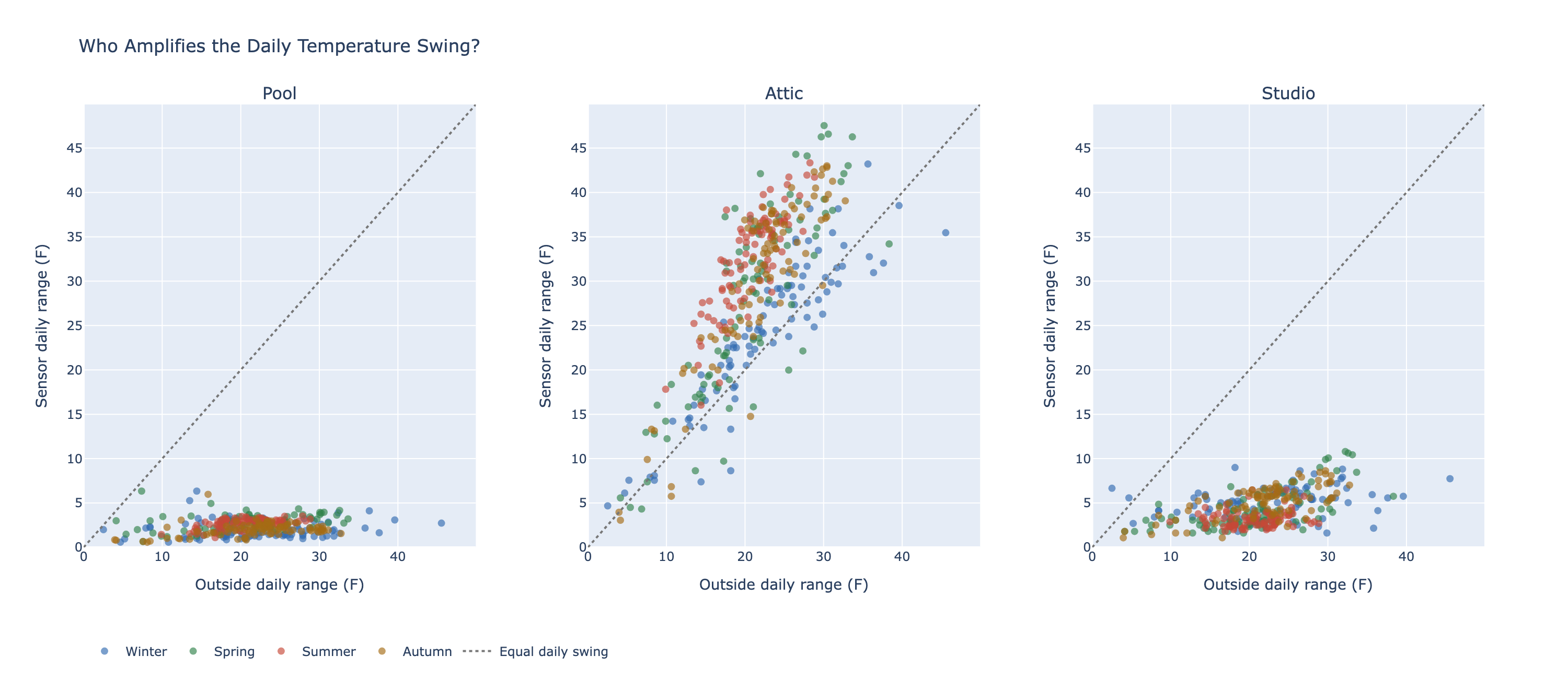
A point above the diagonal has a larger daily range than Outside; one below it has a smaller range. All three panels use the same axes and seasonal colors.
The Attic’s temperature range exceeded Outside’s on about 88% of days. The Pool’s range did not exceed Outside’s on any day, and the Studio’s did so only rarely. But interestingly, the temperature ranges were generally smaller (more smashed to the bottom) for the Pool than for the Studio. The thermal inertia of the Pool was greater than the thermal inertia of my Studio (as provided by my HVAC system).
A Clock for Each Month
These polar charts put clock time around a circle, with midnight at the top and the hours moving clockwise. Each monthly line follows the mean temperature at each hour; all panels use the same radial temperature scale.
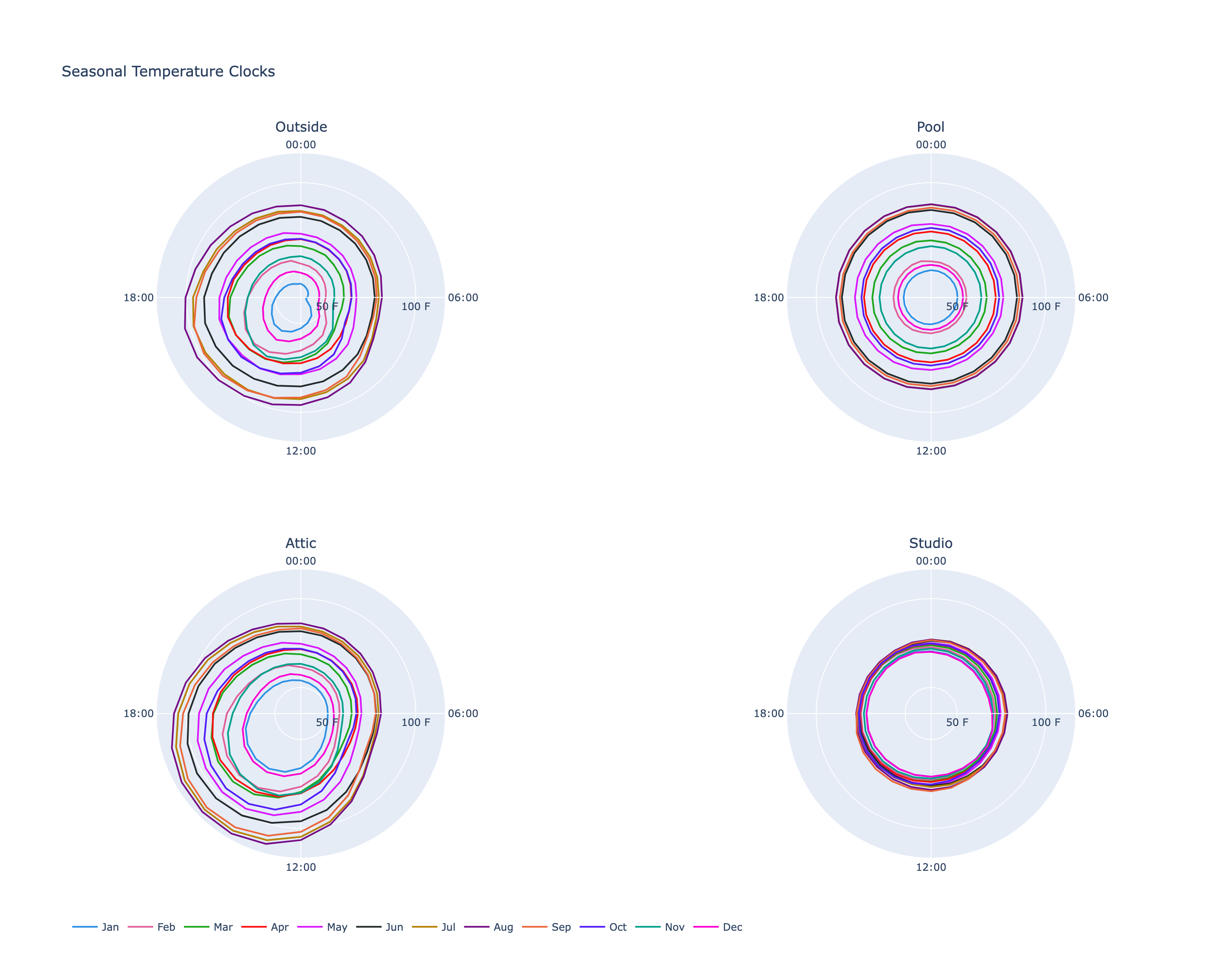
Increasing temperature grows ‘outward’. The curves close at midnight to make the daily cycle easier to see.
The shape shows the typical within-day cycle for each month, while the radius reflects its temperature level. It is a compact way to compare both season and time of day.
Summary
Outside has large daily and seasonal changes. The Attic often amplifies the daytime heat. The Studio stays within a comparatively narrow range. And the Pool responds on a slower schedule, carrying yesterday’s weather into today.
None of that is especially surprising in principle. But there is something satisfying about watching familiar physical ideas emerge from months of measurements taken around your own home.
And yes, I still like data.